Training Neural Networks: Backpropagation and Gradient Descent

Loss Functions

Loss functions measure how far the network's predictions are from the actual values. They quantify the error in the model's predictions, and the goal of training is to minimize this error.

Common loss functions include:

Mean Squared Error (MSE): Used for regression problems
```
L = (1/n) * Σ(y_pred - y_true)²
```

Binary Cross-Entropy: Used for binary classification

L = -(1/n) * Σ[y_true*log(y_pred) + (1-y_true)*log(1-y_pred)]

Categorical Cross-Entropy: Used for multi-class classification
```
L = -(1/n) * Σ Σ y_true_ij * log(y_pred_ij)
```

The choice of loss function depends on the type of problem you're solving. The goal of training is to find weights that minimize the loss function, and calculus helps us find this minimum by computing the gradient of the loss function with respect to the weights.

Backpropagation

Backpropagation is the algorithm used to compute gradients in neural networks. It works by propagating the error backward through the network, using the chain rule to compute how each weight contributes to the error.

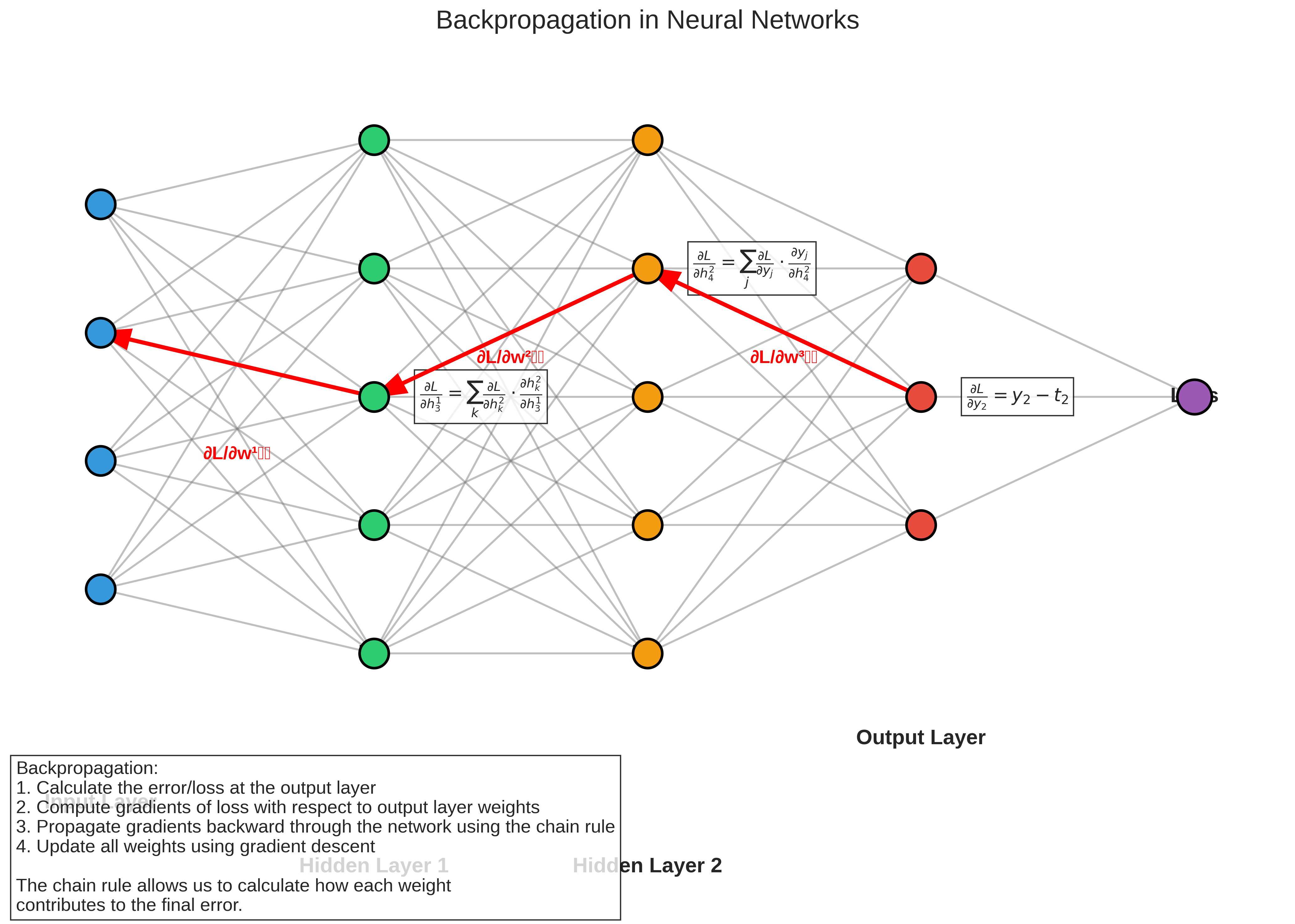
Backpropagation uses the chain rule to efficiently compute gradients

The key insight of backpropagation is that we can efficiently compute the gradient of the loss function with respect to each weight by working backward from the output layer to the input layer, reusing intermediate calculations.

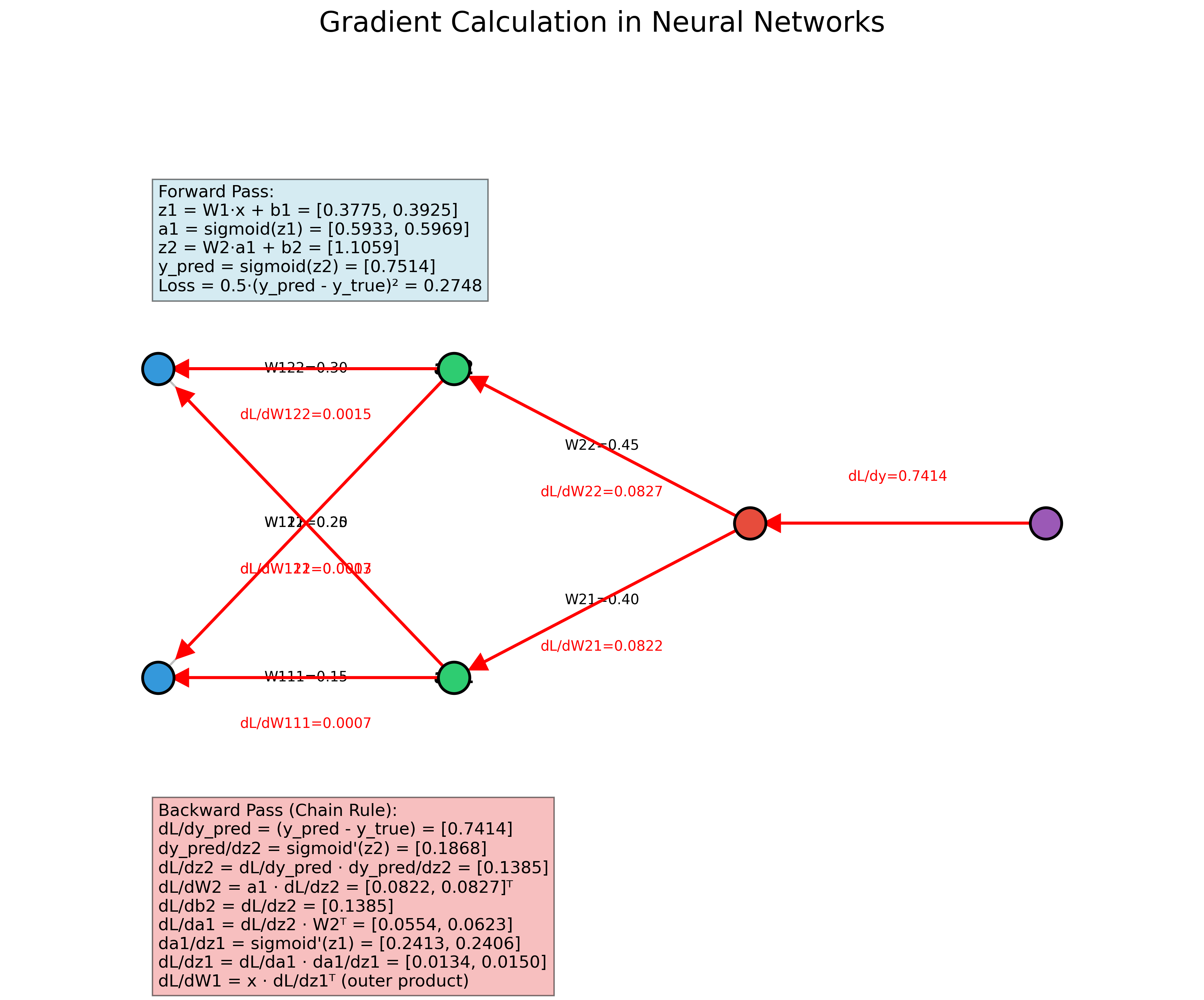
Detailed calculation of gradients using the chain rule

This diagram shows the detailed calculation of gradients in a simple neural network. We start by computing the error at the output layer, then use the chain rule to propagate this error backward through the network. This gives us the gradient of the loss function with respect to each weight, which we use to update the weights.

Backpropagation Algorithm

The backpropagation algorithm consists of the following steps:

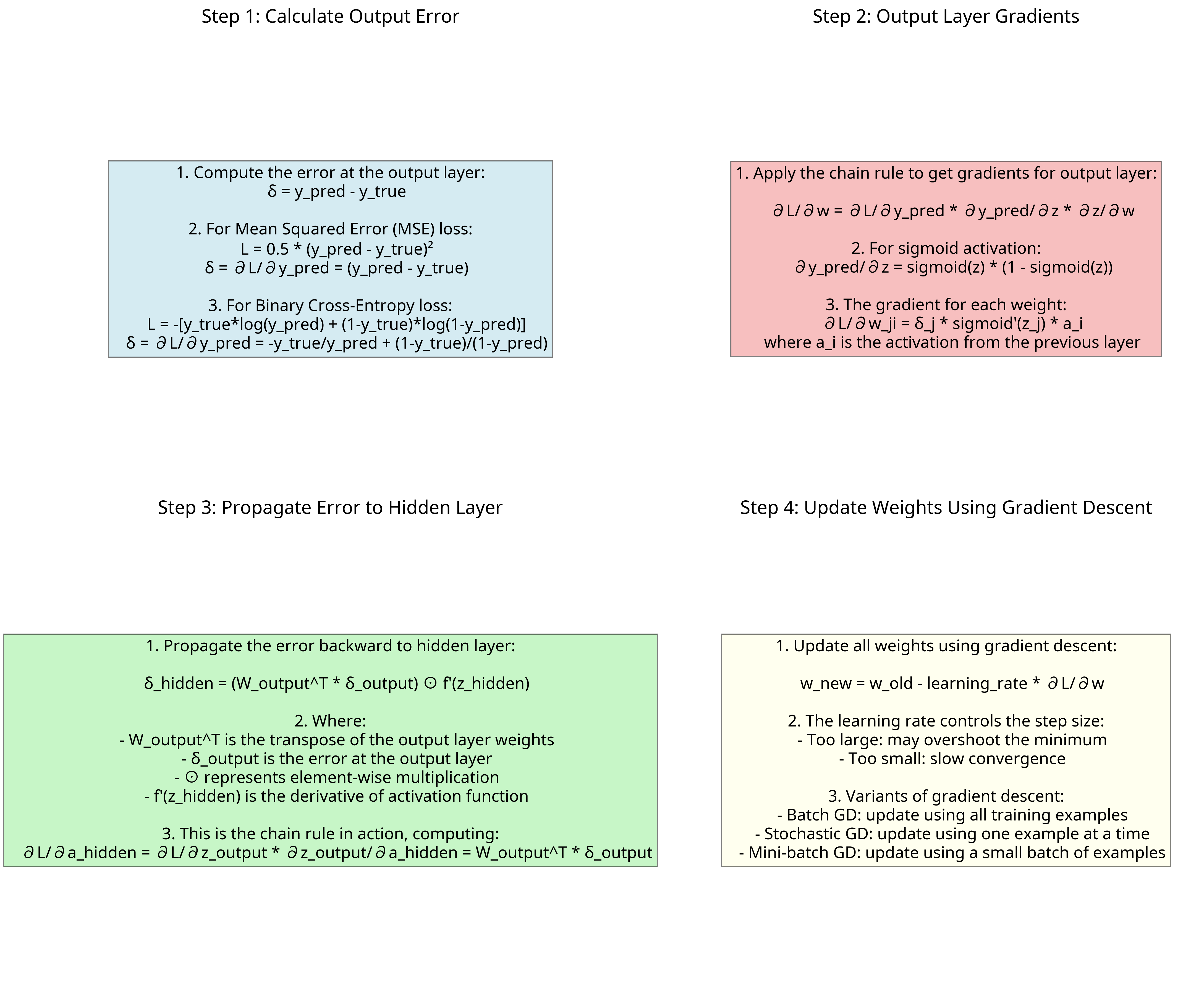
Step-by-step process of backpropagation

Forward Pass: Compute the output of the network for a given input
Compute Loss: Calculate the error between the predicted output and the actual output
Backward Pass:
- Compute the gradient of the loss with respect to the output layer weights
- Propagate the gradients backward through the network using the chain rule
- Compute the gradient of the loss with respect to each weight in the network
Update Weights: Adjust the weights using gradient descent to minimize the loss

Mathematically, for a neural network with L layers, the backpropagation algorithm can be represented as:

# Forward pass
A⁰ = X
For l = 1 to L:
    Z^l = A^(l-1)W^l + b^l
    A^l = σ^l(Z^l)
Y_pred = A^L

# Compute loss
L = loss_function(Y_pred, Y_true)

# Backward pass
dA^L = ∂L/∂A^L
For l = L to 1:
    dZ^l = dA^l * σ'^l(Z^l)
    dW^l = (1/m) * (A^(l-1))^T * dZ^l
    db^l = (1/m) * sum(dZ^l, axis=0)
    if l > 1:
        dA^(l-1) = dZ^l * (W^l)^T

# Update weights
For l = 1 to L:
    W^l = W^l - learning_rate * dW^l
    b^l = b^l - learning_rate * db^l

Where:

dA^l is the gradient of the loss with respect to the activation of layer l
dZ^l is the gradient of the loss with respect to the pre-activation of layer l
dW^l is the gradient of the loss with respect to the weights of layer l
db^l is the gradient of the loss with respect to the biases of layer l
σ'^l is the derivative of the activation function for layer l
m is the number of training examples

Gradient Descent Optimization

Once we have computed the gradients using backpropagation, we use gradient descent to update the weights in a way that minimizes the loss function.

The basic update rule for gradient descent is:

θ = θ - α * ∇J(θ)

Where:

θ represents the parameters (weights and biases)
α is the learning rate (step size)
∇J(θ) is the gradient of the loss function with respect to the parameters

There are several variants of gradient descent:

Batch Gradient Descent: Computes the gradient using the entire dataset
Stochastic Gradient Descent (SGD): Computes the gradient using a single training example
Mini-batch Gradient Descent: Computes the gradient using a small batch of training examples

Advanced optimization algorithms like Adam, RMSprop, and Adagrad build on the basic gradient descent algorithm by adapting the learning rate for each parameter based on historical gradient information.

The Role of Calculus in Training

Calculus plays a crucial role in training neural networks:

Partial Derivatives: Used to compute how each weight affects the loss
Chain Rule: Enables efficient computation of gradients through multiple layers
Gradient Vectors: Provide the direction of steepest descent for optimization
Optimization Theory: Guides the search for minima in the loss landscape

Without calculus, particularly the chain rule and partial differentiation, training deep neural networks would be computationally infeasible. These mathematical concepts are what make deep learning possible.