Code Examples and Implementations
Simple Neural Network Implementation
Below is a complete implementation of a simple neural network from scratch using NumPy. This implementation demonstrates the mathematical concepts we've discussed, including forward propagation, backpropagation, and gradient descent.
import numpy as np
import matplotlib.pyplot as plt

class SimpleNeuralNetwork:
    def __init__(self, input_size, hidden_size, output_size, learning_rate=0.01):
        """
        Initialize a simple neural network with one hidden layer

        Parameters:
        - input_size: number of input features
        - hidden_size: number of neurons in the hidden layer
        - output_size: number of output neurons
        - learning_rate: learning rate for gradient descent
        """
        self.input_size = input_size
        self.hidden_size = hidden_size
        self.output_size = output_size
        self.learning_rate = learning_rate

        # Initialize weights and biases with random values
        # Xavier/Glorot initialization for better gradient flow
        self.W1 = np.random.randn(input_size, hidden_size) * np.sqrt(1 / input_size)
        self.b1 = np.zeros((1, hidden_size))
        self.W2 = np.random.randn(hidden_size, output_size) * np.sqrt(1 / hidden_size)
        self.b2 = np.zeros((1, output_size))

        # For tracking loss during training
        self.loss_history = []

    def sigmoid(self, x):
        """Sigmoid activation function: 1 / (1 + exp(-x))"""
        # Clip x to avoid overflow
        x = np.clip(x, -500, 500)
        return 1 / (1 + np.exp(-x))

    def sigmoid_derivative(self, x):
        """Derivative of sigmoid: sigmoid(x) * (1 - sigmoid(x))"""
        s = self.sigmoid(x)
        return s * (1 - s)

    def forward(self, X):
        """
        Forward propagation through the network

        Parameters:
        - X: input data of shape (batch_size, input_size)

        Returns:
        - Tuple containing:
          - y_pred: output predictions
          - cache: cached values for backpropagation
        """
        # First layer: input to hidden
        # z1 = X·W1 + b1 (matrix multiplication)
        z1 = np.dot(X, self.W1) + self.b1

        # Apply activation function
        a1 = self.sigmoid(z1)

        # Second layer: hidden to output
        # z2 = a1·W2 + b2 (matrix multiplication)
        z2 = np.dot(a1, self.W2) + self.b2

        # Apply sigmoid activation for output layer
        y_pred = self.sigmoid(z2)

        # Cache values for backpropagation
        cache = {
            'X': X,
            'z1': z1,
            'a1': a1,
            'z2': z2,
            'y_pred': y_pred
        }

        return y_pred, cache

    def compute_loss(self, y_pred, y_true):
        """
        Compute binary cross-entropy loss

        Parameters:
        - y_pred: predicted values
        - y_true: true values

        Returns:
        - loss: scalar loss value
        """
        # Binary cross-entropy loss
        # L = -1/m * Σ[y·log(ŷ) + (1-y)·log(1-ŷ)]
        m = y_true.shape[0]

        # Add small epsilon to avoid log(0)
        epsilon = 1e-15
        y_pred = np.clip(y_pred, epsilon, 1 - epsilon)

        loss = -1/m * np.sum(y_true * np.log(y_pred) + (1 - y_true) * np.log(1 - y_pred))
        return loss

    def backward(self, y_pred, y_true, cache):
        """
        Backward propagation to compute gradients

        Parameters:
        - y_pred: predicted values
        - y_true: true values
        - cache: cached values from forward propagation

        Returns:
        - gradients: dictionary containing gradients for W1, b1, W2, b2
        """
        m = y_true.shape[0]

        # Get cached values
        X = cache['X']
        z1 = cache['z1']
        a1 = cache['a1']

        # Output layer gradient
        # dL/dz2 = (y_pred - y_true) * sigmoid_derivative(z2)
        # For binary cross-entropy with sigmoid, this simplifies to (y_pred - y_true)
        dz2 = y_pred - y_true

        # Gradient for W2: dL/dW2 = a1^T · dz2
        dW2 = 1/m * np.dot(a1.T, dz2)

        # Gradient for b2: dL/db2 = sum(dz2)
        db2 = 1/m * np.sum(dz2, axis=0, keepdims=True)

        # Hidden layer gradient using chain rule
        # dL/da1 = dz2 · W2^T
        da1 = np.dot(dz2, self.W2.T)

        # dL/dz1 = dL/da1 * sigmoid_derivative(z1)
        dz1 = da1 * self.sigmoid_derivative(z1)

        # Gradient for W1: dL/dW1 = X^T · dz1
        dW1 = 1/m * np.dot(X.T, dz1)

        # Gradient for b1: dL/db1 = sum(dz1)
        db1 = 1/m * np.sum(dz1, axis=0, keepdims=True)

        # Return gradients
        gradients = {
            'dW1': dW1,
            'db1': db1,
            'dW2': dW2,
            'db2': db2
        }

        return gradients

    def update_parameters(self, gradients):
        """
        Update parameters using gradient descent

        Parameters:
        - gradients: dictionary containing gradients for W1, b1, W2, b2
        """
        # Update weights and biases
        # W = W - learning_rate * dW
        self.W1 -= self.learning_rate * gradients['dW1']
        self.b1 -= self.learning_rate * gradients['db1']
        self.W2 -= self.learning_rate * gradients['dW2']
        self.b2 -= self.learning_rate * gradients['db2']

    def train(self, X, y, epochs=1000, print_every=100):
        """
        Train the neural network

        Parameters:
        - X: input data
        - y: target values
        - epochs: number of training iterations
        - print_every: print loss every n epochs

        Returns:
        - loss_history: list of loss values during training
        """
        self.loss_history = []

        for i in range(epochs):
            # Forward propagation
            y_pred, cache = self.forward(X)

            # Compute loss
            loss = self.compute_loss(y_pred, y)
            self.loss_history.append(loss)

            # Backward propagation
            gradients = self.backward(y_pred, y, cache)

            # Update parameters
            self.update_parameters(gradients)

            # Print loss every n epochs
            if i % print_every == 0:
                print(f"Epoch {i}, Loss: {loss:.4f}")

        return self.loss_history

    def predict(self, X):
        """
        Make predictions

        Parameters:
        - X: input data

        Returns:
        - predictions: binary predictions (0 or 1)
        """
        # Forward propagation
        y_pred, _ = self.forward(X)

        # Convert probabilities to binary predictions
        predictions = (y_pred > 0.5).astype(int)

        return predictions
This implementation includes all the key components of a neural network:
- Initialization of weights and biases
- Forward propagation to make predictions
- Loss computation to measure error
- Backpropagation to compute gradients
- Parameter updates using gradient descent
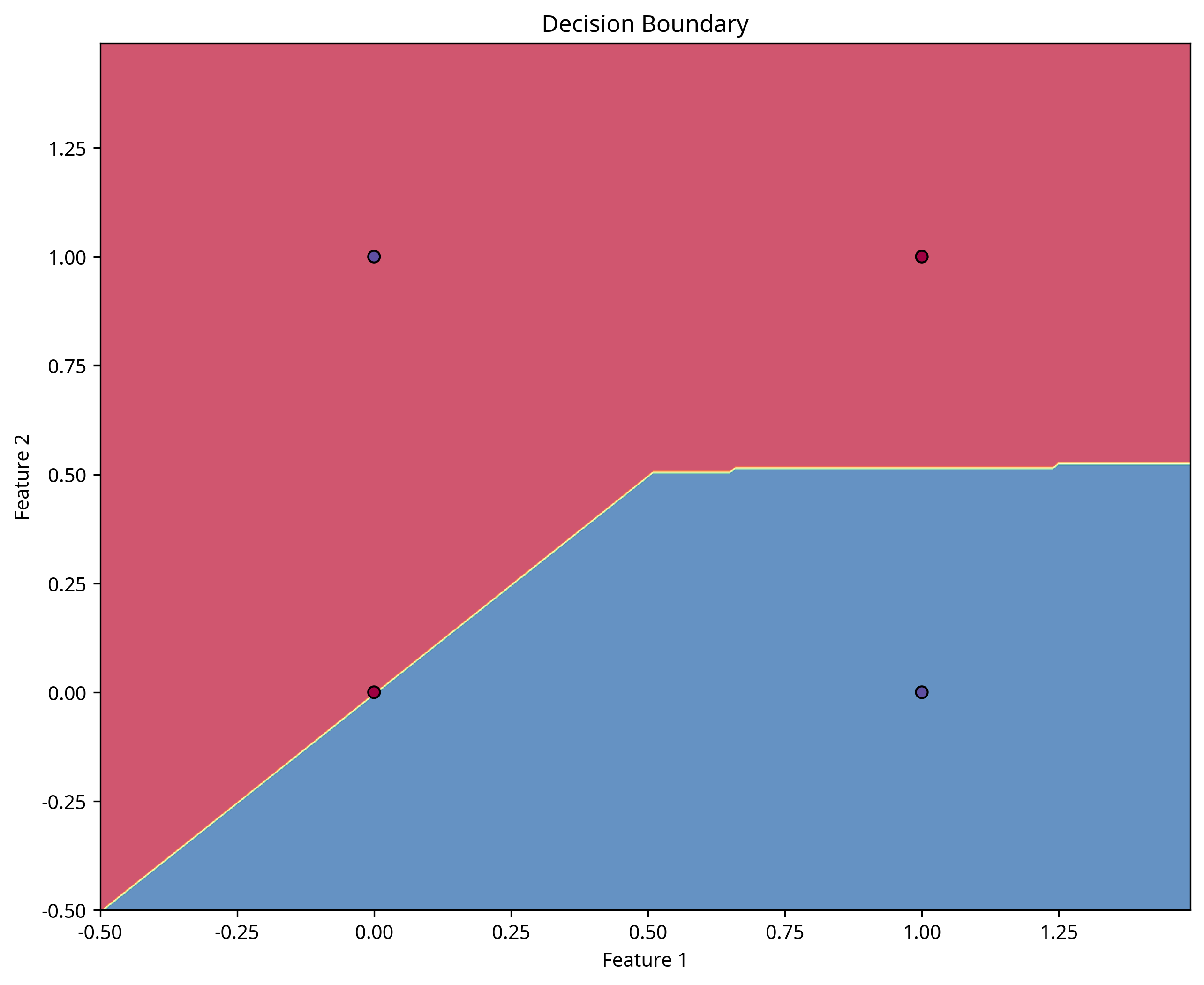
Decision boundary learned by a neural network for the XOR problem
The image above shows the decision boundary learned by a neural network for the XOR problem, which is not linearly separable. This demonstrates the power of neural networks to learn complex patterns.
Forward Propagation Example
Here's a simplified example of forward propagation in a neural network:
# Forward propagation in a neural network
def forward(X, W1, b1, W2, b2):
    # First layer: input to hidden
    z1 = np.dot(X, W1) + b1  # Matrix multiplication
    a1 = sigmoid(z1)         # Apply activation function

    # Second layer: hidden to output
    z2 = np.dot(a1, W2) + b2 # Matrix multiplication
    y_pred = sigmoid(z2)     # Apply activation function

    return y_pred, (z1, a1, z2)
This code shows the forward propagation process in a neural network. We compute the weighted sum of inputs (z), then apply an activation function to get the activation (a). This process is repeated for each layer. The final output is our prediction.
Backpropagation Example
Here's a simplified example of backpropagation in a neural network:
# Backward propagation to compute gradients
def backward(X, y, y_pred, cache, W1, W2):
    z1, a1, z2 = cache
    m = X.shape[0]

    # Output layer gradient
    dz2 = y_pred - y                  # Derivative of loss w.r.t. z2
    dW2 = (1/m) * np.dot(a1.T, dz2)   # Gradient for W2
    db2 = (1/m) * np.sum(dz2, axis=0) # Gradient for b2

    # Hidden layer gradient (chain rule)
    da1 = np.dot(dz2, W2.T)           # dL/da1 = dL/dz2 · dz2/da1
    dz1 = da1 * sigmoid_derivative(z1)# dL/dz1 = dL/da1 · da1/dz1
    dW1 = (1/m) * np.dot(X.T, dz1)    # Gradient for W1
    db1 = (1/m) * np.sum(dz1, axis=0) # Gradient for b1

    return dW1, db1, dW2, db2
This code implements the backpropagation algorithm. We start by computing the gradient at the output layer, then use the chain rule to propagate this gradient backward through the network. Notice how we compute the gradient for each weight and bias.
Gradient Descent Update Example
Here's a simplified example of gradient descent update in a neural network:
# Update parameters using gradient descent
def update_parameters(W1, b1, W2, b2, dW1, db1, dW2, db2, learning_rate):
    W1 = W1 - learning_rate * dW1  # Update weights for layer 1
    b1 = b1 - learning_rate * db1  # Update biases for layer 1
    W2 = W2 - learning_rate * dW2  # Update weights for layer 2
    b2 = b2 - learning_rate * db2  # Update biases for layer 2

    return W1, b1, W2, b2
This code shows how we update the parameters using gradient descent. We subtract the gradient multiplied by the learning rate from each parameter. This moves the parameters in the direction of steepest descent, reducing the loss function.
Visualizing Gradient Descent
The following code generates visualizations of gradient descent optimization on a loss surface:
import numpy as np
import matplotlib.pyplot as plt
from matplotlib.colors import LinearSegmentedColormap
from mpl_toolkits.mplot3d import Axes3D

# Define a loss function (a simple quadratic function)
def loss_function(w1, w2):
    return w1**2 + w2**2 + 2*w1*w2 + 2

# Define the gradient of the loss function
def gradient(w1, w2):
    dw1 = 2*w1 + 2*w2
    dw2 = 2*w2 + 2*w1
    return np.array([dw1, dw2])

# Implement gradient descent
def gradient_descent(start_w1, start_w2, learning_rate, num_iterations):
    w1, w2 = start_w1, start_w2
    path_w1, path_w2, path_z = [w1], [w2], [loss_function(w1, w2)]

    for i in range(num_iterations):
        grad = gradient(w1, w2)
        w1 = w1 - learning_rate * grad[0]
        w2 = w2 - learning_rate * grad[1]
        path_w1.append(w1)
        path_w2.append(w2)
        path_z.append(loss_function(w1, w2))

    return np.array(path_w1), np.array(path_w2), np.array(path_z)

# Create a 3D visualization of the loss function with gradient descent paths
fig = plt.figure(figsize=(14, 10))
ax = fig.add_subplot(111, projection='3d')

# Create a meshgrid for the parameter space
w1 = np.linspace(-4, 4, 100)
w2 = np.linspace(-4, 4, 100)
W1, W2 = np.meshgrid(w1, w2)
Z = loss_function(W1, W2)

# Plot the loss surface
surf = ax.plot_surface(W1, W2, Z, cmap='viridis', alpha=0.8, linewidth=0)

# Run gradient descent with different learning rates
start_w1, start_w2 = 3.5, 3.5
learning_rates = [0.01, 0.05, 0.1, 0.2]
num_iterations = 50

# Plot gradient descent paths with different learning rates
for lr in learning_rates:
    path_w1, path_w2, path_z = gradient_descent(start_w1, start_w2, lr, num_iterations)
    ax.plot(path_w1, path_w2, path_z, 'o-', linewidth=2, markersize=4, label=f'Learning Rate = {lr}')

# Add labels and title
ax.set_xlabel('Weight 1')
ax.set_ylabel('Weight 2')
ax.set_zlabel('Loss')
ax.set_title('Gradient Descent Optimization on Loss Surface', fontsize=16)

# Add a legend
ax.legend(loc='upper right')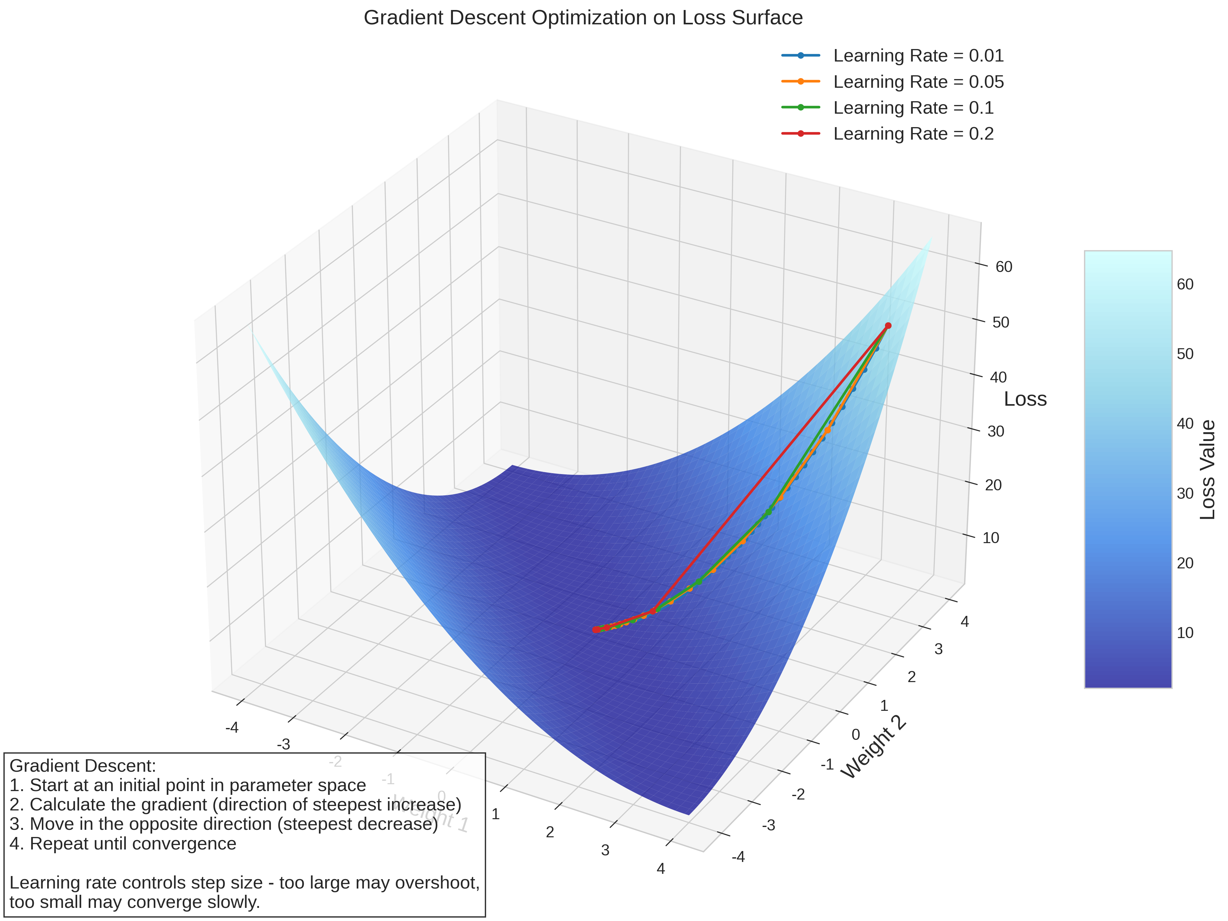
3D visualization of gradient descent optimization on a loss surface
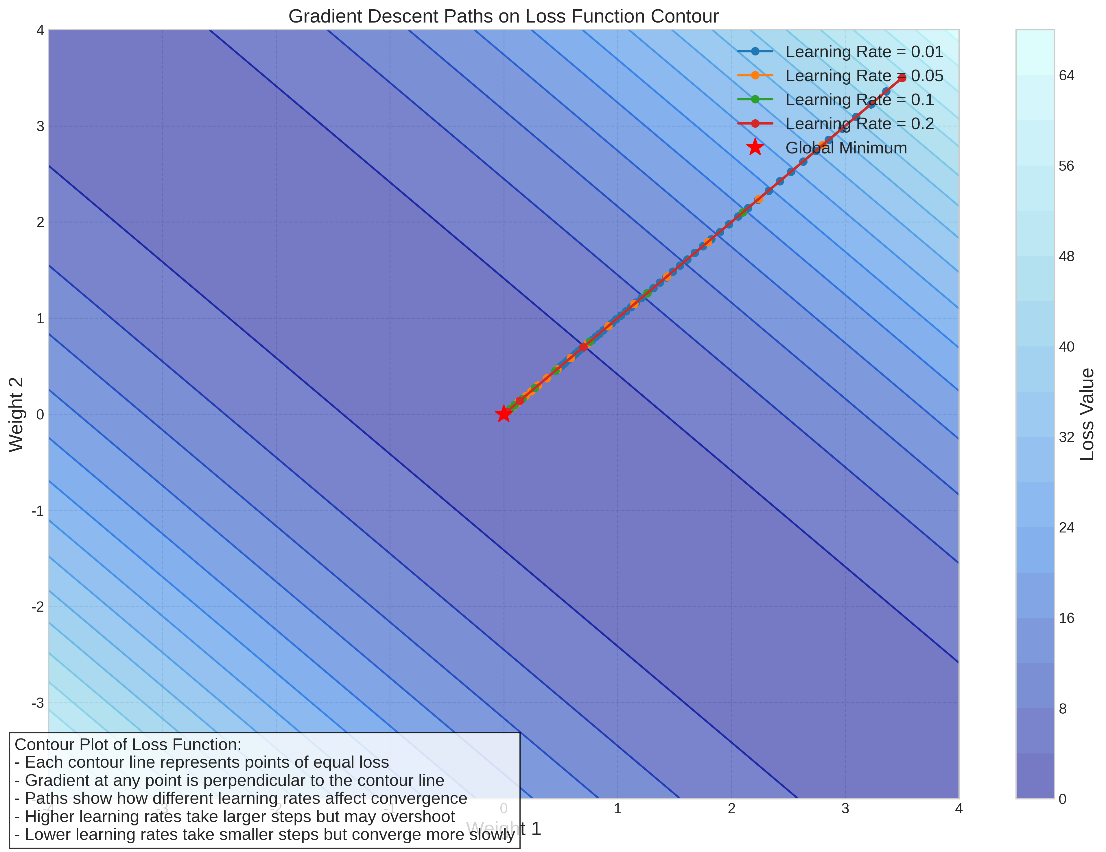
Contour plot showing gradient descent paths with different learning rates